Appendix B — Appendix: Sample Event Timing

B.1 Introduction

Sample event timing for spring and summer events must be chosen with care each year. Sample date occurs on Tuesdays traditionally, and dates must be chosen such that the tide is incoming early in the morning.

B.1.0.0.1 Notes on data sourcing

Data is sourced from the following queries at https://waterqualitydata.us on Feb 24, 2021:

CSV download for sample data: https://www.waterqualitydata.us/portal/#bBox=-151.322501%2C60.274310%2C-149.216144%2C60.738915&mimeType=csv&dataProfile=narrowResult

CSV download for site data: https://www.waterqualitydata.us/portal/#countrycode=US&statecode=US%3A02&countycode=US%3A02%3A122&bBox=-151.322501%2C60.274310%2C-149.216144%2C60.738915&mimeType=csv

Note: these CSV files are excluded from the GitHub repository because they are too large to sync. To reproduce the analysis, download and save these files locally instead. (See the ReadMe file at data/WQX_downloads in the repository).

Using these same queries in the future will download the most current csv files.

---

B.1.1 Import data

Import data from local csv files

Code

# read in table of known dates from Guerron Orejuela 2016
krbwqm_dates <- read_excel("other/input/sample_dates_tides.xlsx") %>%
  rename(activity_start_date = date) %>%
  transform(time_max_tide = as.hms(time_max_tide),
            time_min_tide = as.hms(time_min_tide)) %>%
  select(-data_entry,-link,-sample_date_source,-tide_source) %>%
  mutate(julian_day = yday(activity_start_date),
         year = year(activity_start_date))

z <- krbwqm_dates %>%
  arrange(season,julian_day)

B.2 Dates

Code

# dot plot
krbwqm_dates %>%
  ggplot(aes(year,julian_day)) +
  geom_point() +
  ggtitle("Kenai River Baseline Water Quality Sampling Dates")

Code

# calculate spring and summer average days
krbwqm_dates %>%
  distinct(julian_day,season,year) %>%
  group_by(season) %>%
  summarise(avg_date = format(as.Date(round(mean(julian_day)), origin = as.Date("2024-01-01")), "%m-%d"),
            stdev = round(sd(julian_day)),
            n_years = n(),
            min_year = min(year),
            max_year = max(year))

# A tibble: 2 × 6
  season avg_date stdev n_years min_year max_year
  <chr>  <chr>    <dbl>   <int>    <dbl>    <dbl>
1 spring 04-27        7      21     2001     2022
2 summer 07-25        4      23     2000     2022

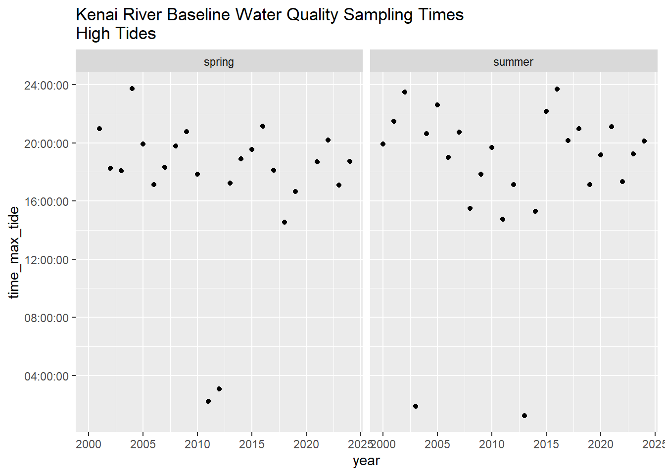
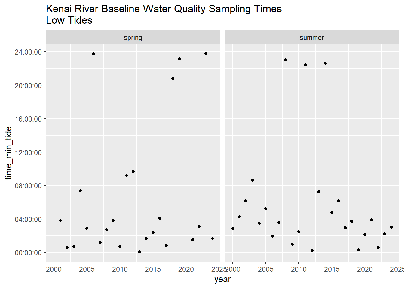
B.3 Time of Day

Code

# dot plot
krbwqm_dates %>%
  ggplot(aes(year,time_max_tide)) +
  geom_point() +
  facet_grid(.~season) +
  ggtitle("Kenai River Baseline Water Quality Sampling Times\nHigh Tides")

Code

krbwqm_dates %>%
  ggplot(aes(year,time_min_tide)) +
  geom_point() +
  facet_grid(.~season) +
  ggtitle("Kenai River Baseline Water Quality Sampling Times\nLow Tides")

Code

# calculate spring and summer average days
krbwqm_dates %>%
  distinct(julian_day,season,year) %>%
  group_by(season) %>%
  summarise(avg_date = format(as.Date(round(mean(julian_day)), origin = as.Date("2024-01-01")), "%m-%d"),
            stdev = round(sd(julian_day)),
            n_years = n(),
            min_year = min(year),
            max_year = max(year))

# A tibble: 2 × 6
  season avg_date stdev n_years min_year max_year
  <chr>  <chr>    <dbl>   <int>    <dbl>    <dbl>
1 spring 04-27        7      21     2001     2022
2 summer 07-25        4      23     2000     2022